Illustrated Excel 2019 | Module 5 End of Module Project 1 | City Sports

Illustrated Excel 2019 | Module 5: End of Module Project 1 #illustratedexcel #Module5 #EOMProject1

If you directly want to get the project from us then contact us on Whatsapp. Click on link below👇👇
https://wa.me/message/PPXGSJS2TLWUA1

Whatsapp Contact Number:
+91 8114420233

Email ID:
[email protected]


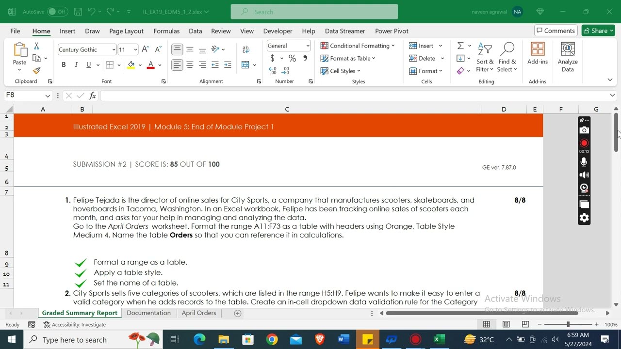
1. "Felipe Tejada is the director of online sales for City Sports, a company that manufactures scooters, skateboards, and hoverboards in Tacoma, Washington. In an Excel workbook, Felipe has been tracking online sales of scooters each month, and asks for your help in managing and analyzing the data.
Go to the April Orders worksheet. Format the range A11:F73 as a table with headers using Orange, Table Style Medium 4. Name the table Orders so that you can reference it in calculations."
Format a range as a table.
Apply a table style.
Set the name of a table.
2. "City Sports sells five categories of scooters, which are listed in the range H5:H9. Felipe wants to make it easy to enter a valid category when he adds records to the table. Create an in-cell dropdown data validation rule for the Category column that accepts only entries from the range H5:H9. Show an input message when the cell is selected using Scooter Category as the title. Use the following sentence as the input message:
Click the arrow to select a category.
Apply an Information style error alert that also uses Scooter Category as the title and the following sentence as the error message:
Please select a category from the list."
Add a data validation rule to a range.
Add an input message to a data validation rule.
Add an error alert to a data validation rule.
3. Felipe needs to show the total billed amount in the Orders table. Insert a table column to the right of the Shipping column. Type Total Billed as the column heading. Resize columns A, F, and G to their best fit to display the full text of the header cells in those columns.
Add a column to a table.
Change the column width.
4. In cell G12, enter a formula without a function that uses structured references to add the Price and Shipping values for the first record. If necessary, fill the range G13:G73 with the formula in cell G12.
Use structured references in a formula.
In the April Orders worksheet, the formula in cell G12 has not been entered correctly.
Copy a formula into a range.
In the April Orders worksheet, the formula in cell G12 has not been entered correctly.
5. Felipe received an online order and needs to add it to the Orders table. Add a new record to the end of the table and then insert the data shown in Table 1, using the in-cell dropdown list to enter the Category value.
Add a record to a table.
6. The table is not currently sorted, but Felipe wants to sort it by the Order Date, with the oldest records listed first, which will help him find orders quickly. For orders received on the same date, he wants to list the orders by Product Name. Sort the table in ascending order first by Order Date and then by Product Name.
Sort a table on multiple ranges.
7. Felipe also wants to track the total billing amount, the average price, and the number of orders. Add a Total row to the Orders table, which automatically sums the amounts in the Total Billed column. In cell B75, use the total row to display the count of the Order IDs. In cell E75, use the total row to display the average Price.
Insert a Total row in a table.
Summarize table data with a total row.
8. Felipe has created a lookup area in the range A4:B7. First, he wants to find the product name associated with the Order ID entered in cell B5. In cell B6, enter a formula using the INDEX and MATCH functions and structured references to the columns in the Orders table. Return a value from the Product Name column that exactly matches the value in cell B5, which is listed in the Order ID column of the Orders table.
Use structured references in a formula.
In the April Orders worksheet, the formula in cell B6 should contain a structured reference to the Product Name column.
9. Next, Felipe wants to find the amount billed for the order entered in cell B5. In cell B7, enter a formula using the VLOOKUP function and structured references to the columns in the Orders table. Look up the value in cell B5, refer to the six columns in the Orders table beginning with Order ID and ending with Total Billed (range B12:G74), and return a value in column 6 that exactly matches the value in cell B5.

#excelproject #excel2019 #module5 #samproject1b #samproject1a #illustratedexcel #eom2 #eom1 #endofmodule #eomproject2