Exp22_Excel_Ch07_CumulativeAssessment_Variation_Shipping | Exp22 Excel Ch07 CumulativeAssessment

For Complete solution of Assignments and for the deal of complete Courses.
Contact Me
WhatsApp : +923209088014
Email : myitlabservice@gmail.com
WhatsApp Direct Link :https://wa.me/923209088014


#Exp22_Excel_Ch07_CumulativeAssessment_Variation_Shipping #Excel_Ch07_CumulativeAssessment_Variation_Shipping #Ch07_CumulativeAssessment_Variation_Shipping
Exp22_Excel_Ch07_CumulativeAssessment_Variation_Shipping | Exp22 Excel Ch07 CumulativeAssessment
#Exp22_Excel_Ch07_CumulativeAssessment_Variation_Shipping#Excel_Ch07_CumulativeAssessment_Variation_Shipping#Ch07_CumulativeAssessment_Variation_Shipping#CumulativeAssessment_Variation_Shipping
#Variation_Shipping#Exp22_Excel_Ch07_CumulativeAssessment_Variation
Exp22_Excel_Ch07_CumulativeAssessment_Shipping

Project Description:
You work for a company that sells cell phone accessories. The company has distribution centers in three states. You want to analyze shipping data for one week in April to determine if shipping times are too long. You will perform other analysis and insert a map. Finally, you will prepare a partial loan amortization table for a new delivery van.
1 Start Excel. Download and open the file named Exp22_Excel_Ch07_CumulativeAssessment_Shipping.xlsx. Grader has automatically added your last name to the beginning of the filename.
2 The Week worksheet contains data for the week of August 5.

In cell D7, insert the appropriate date function to calculate the number of days between the Date Arrived and Date Ordered. Copy the function to the range D8:D35.

Hint: Formula is =DAYS(Date Arrived, Date Ordered)
3 You want to display the weekday for the arrival dates.

In cell E7, insert the WEEKDAY function to identify an integer representing the weekday of the Date Arrived. Copy the function to the range E8:E35.
Hint: Formula is =WEEKDAY(Date Arrived).
4 You need to format the WEEKDAY function results with a custom number format.

Select the range E7:E35, apply the custom number format dddd, and apply center horizontal alignment.
5 Next, you want to display the city names that correspond with the city airport codes.

In cell G7, insert the SWITCH function to evaluate the airport code in cell E7. Include mixed cell references to the city names in the range G2:G4. Use the airport codes as text for the Value arguments: AUS for Austin, DFW for Dallas-Fort Worth, and IAH for Houston. Copy the function to the range G8:G35.

Hint: Formula is =SWITCH(Airport Code, AUS, cell reference to Austin, DFW, cell reference to Dallas-Fort Worth, IAH, cell reference to Houson)
6 Now you want to display the standard shipping costs by city.

In cell I7, insert the IFS function to identify the shipping cost based on the airport code and the applicable shipping rates in the range H2:H4. Enter the airport codes in this sequence: AUS, DFW, IAH (with their respective costs). Use relative and mixed references correctly. Copy the function to the range I8:I35.

Hint: Formula is =IFS(Airport Code = AUS, cell reference to $24, Airport Code = DFW, cell reference to $20, Airport Code = IAH, cell reference to $30)
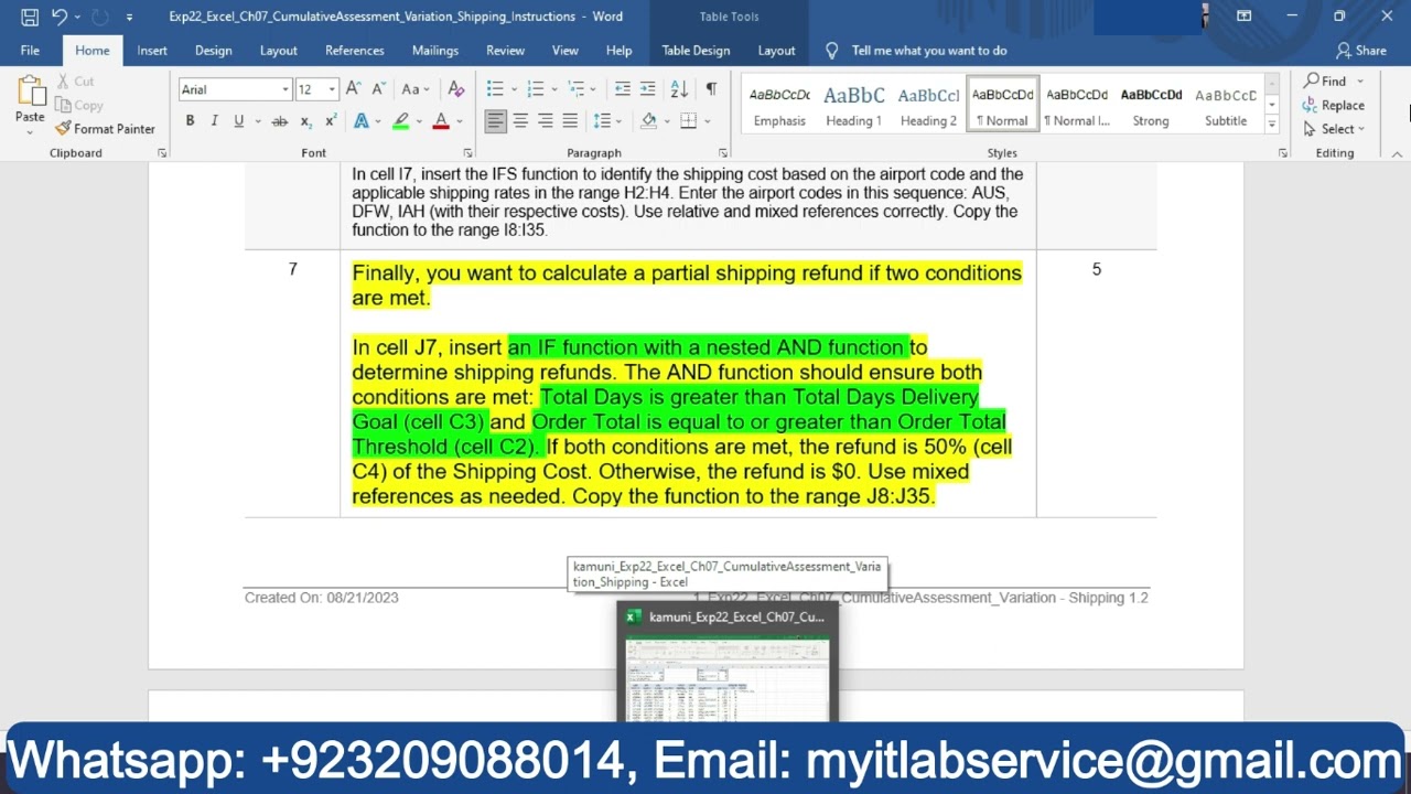
7 Finally, you want to calculate a partial shipping refund if two conditions are met.

In cell J7, insert an IF function with a nested AND function to determine shipping refunds. The AND function should ensure both conditions are met: Total Days is greater than Total Days Delivery Goal (cell C3) and Order Total is equal to or greater than Order Total Threshold (cell C2). If both conditions are met, the refund is 50% (cell C4) of the Shipping Cost. Otherwise, the refund is $0. Use mixed references as needed. Copy the function to the range J8:J35.

Hint: Formula is =IF(AND(Total Days greater than 7, Order Total greater than or equal to $1,000), Shipping Cost*50%, 0)
8 The Stats worksheet contains similar data. Now you want to enter summary statistics.

In cell B2, insert the COUNTIF function to count the number of shipments for Austin (cell B1). Use appropriate mixed references to the range argument to keep the column letters the same. Copy the function to the range C2:D2.

Hint: Formula is =COUNTIF(Airport Code, AUS)
9 In cell B3, insert the SUMIF function to calculate the total orders for Austin (cell B1). Use appropriate mixed references to the range argument to keep the column letters the same. Copy the function to the range C3:D3.

Hint: Formula is =SUMIF(Airport Code column, AUS, Order Total column)
10 In cell B4, insert the AVERAGEIF function to calculate the average number of days for shipments from Austin (cell B1). Use appropriate mixed references to the range argument to keep the column letters the same. Copy the function to the range C4:D4.

Hint: Formula is =AVERAGEIF(Airport Code column, AUS, Total Days column)
11 Now you want to focus on shipments from Houston where the order was greater than $1,000.