FEA Isoparametric Quadrilaterals Part 3: Gauss Quadrature for Integration of the Stiffness Matrix

This video continues from part 1 (   • FEA Isoparametric Quadrilaterals Part 1: J...  ) and part 2 (   • FEA Isoparametric Quadrilaterals Part 2: T...  ) to investigate how to integrate the stiffness matrix for linear 4-node isoparametric quadrilateral elements in finite element analysis (FEA). This video shows how Gauss quadrature can be used to transform the integration of [K] into summation of the integrand within [K] evaluated at four distinct locations called Gauss points, integration points, and/or sampling points.

0:00 Introduction and review of the elemental stiffness matrix equation
1:05 Why direct integration of the stiffness matrix would be difficult
2:02 Introduction to Gauss quadrature
3:57 Table of sampling points for Gauss quadrature (also called Gauss points or integration points)
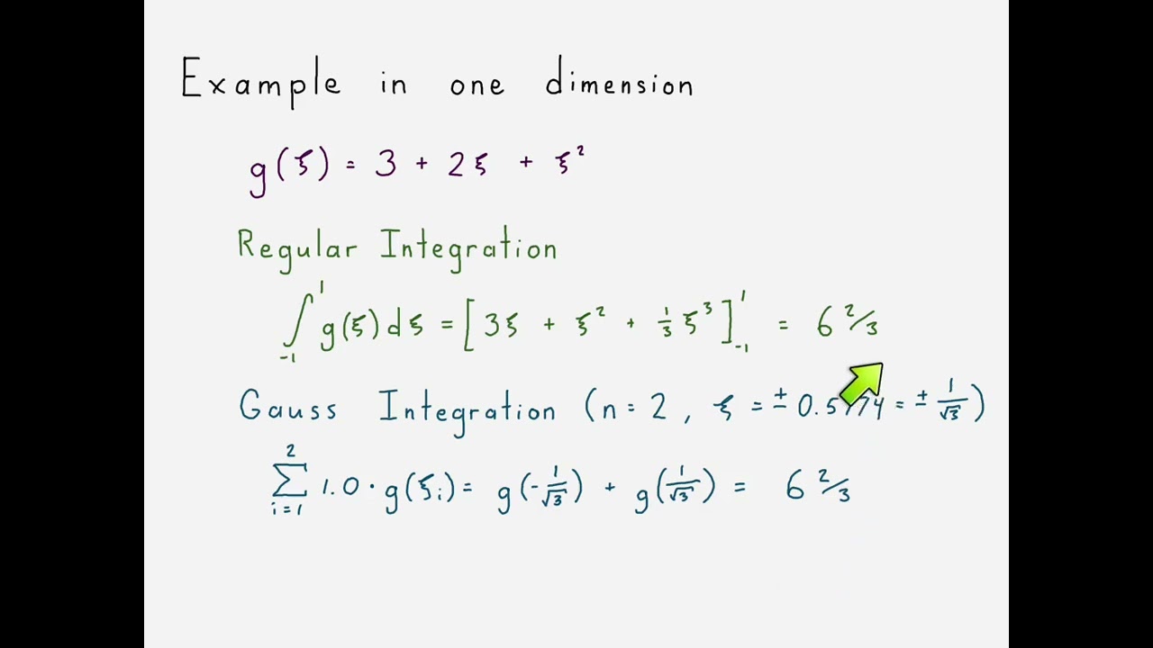
5:14 Gauss quadrature example with one variable (1D)
6:40 Gauss quadrature example with two variables (2D)
8:45 Gauss quadrature applied to the elemental stiffness matrix equation for 4-node linear isoparametric quadrilateral
10:20 Reflection questions

Suggested answers to the reflection questions
1.) The main advantage of Gauss quadrature is that it changes the integral of a polynomial into summation of that polynomial integrated at distinct locations (called Gauss points, integration points, or sampling points)
2.) Gauss quadrature works most easily on the interval between -1 and 1 although there are techniques for it to work over other interval ranges. Gauss quadrature will give the exact integral result for polynomials of order k as long as the polynomial is evaluated at a sufficient number of Gauss integration points, n. The order of the polynomial, k must be less than or equal to 2n-1 for exact representation. If less Gauss points are used, then it will give an approximate representation (this is done sometimes in FEA for reduced integration).
3.) n = 2 is sufficient in each direction for integrating the 4-node linear isoparametric element because each component of the integrand matrix equation (transpose[B]*[C]*[B]*|J|) would at most be a cubic polynomial in either xi or eta directions (k = 3 = 2n-1).
4.) The four Gauss integration points are located at:
xi = -1/sqrt(3), eta = -1/sqrt(3)
xi = 1/sqrt(3), eta = -1/sqrt(3)
xi = 1/sqrt(3), eta = 1/sqrt(3)
xi = -1/sqrt(3), eta = 1/sqrt(3)